
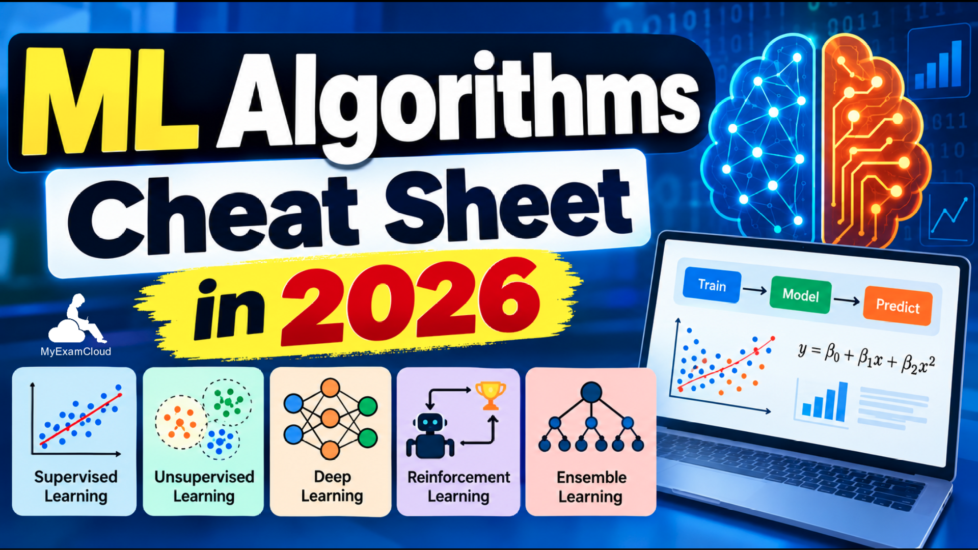
ML Algorithms Cheat Sheet in 2026: A Complete Guide to Machine Learning Algorithms
Read this MyExamCloud Blog article for practical insights on Machine Learning. Explore more blog categories, search related topics in blog search, or return to the MyExamCloud Blog home.
Machine learning has evolved rapidly, with classical statistical algorithms now working alongside deep learning, transformers, generative AI, reinforcement learning, and modern MLOps systems. For students, developers, data analysts, data scientists, and AI engineers, understanding which machine learning algorithm to use—and why—is one of the most important practical skills.
This ML Algorithms Cheat Sheet in 2026 provides a structured reference to the most important machine learning algorithms, their use cases, strengths, limitations, mathematical foundations, and practical considerations.
1. Machine Learning Algorithm Categories
Machine learning algorithms can broadly be divided into the following categories:
| Category | Typical Algorithms | Primary Use |
|---|---|---|
| Supervised Learning | Linear Regression, Logistic Regression, Decision Trees, Random Forest, SVM | Prediction using labeled data |
| Unsupervised Learning | K-Means, DBSCAN, PCA, Hierarchical Clustering | Finding patterns in unlabeled data |
| Semi-Supervised Learning | Self-training, Label Propagation, Pseudo-labeling | Learning with limited labeled data |
| Self-Supervised Learning | Contrastive Learning, Masked Prediction | Learning representations from unlabeled data |
| Deep Learning | CNN, RNN, LSTM, Transformer | Complex representation learning |
| Reinforcement Learning | Q-Learning, DQN, Policy Gradient | Sequential decision making |
| Ensemble Learning | Random Forest, AdaBoost, Gradient Boosting, XGBoost | Combining multiple models |
2. Supervised Learning
Supervised learning learns a mapping between input variables and known target values.
Given training examples:
\(\mathcal{D} = \{(x_1,y_1),(x_2,y_2),\ldots,(x_n,y_n)\}\)
the objective is to learn a function:
\(f(x) \rightarrow y\)
Supervised learning is primarily divided into regression and classification.
3. Linear Regression
Linear Regression predicts a continuous numerical value from one or more input variables.
Simple Linear Regression
\(y = \beta_0 + \beta_1x\)
where:
- y = predicted value
- β0 = intercept
- β1 = coefficient
- x = input feature
Multiple Linear Regression
\(y = \beta_0 + \beta_1x_1 + \beta_2x_2 + \cdots + \beta_px_p\)
A common objective function is Mean Squared Error:
\(MSE = \frac{1}{n}\sum_{i=1}^{n}(y_i-\hat{y}_i)^2\)
Common Applications
- House-price prediction
- Revenue forecasting
- Demand prediction
- Risk modeling
- Trend analysis
4. Polynomial Regression
Polynomial Regression extends linear regression by adding polynomial features.
\(y = \beta_0 + \beta_1x + \beta_2x^2 + \cdots + \beta_dx^d\)
It can model nonlinear relationships while still using a linear regression framework.
5. Ridge Regression
Ridge Regression adds an L2 regularization penalty to reduce overfitting.
\(J(\beta)=MSE+\lambda\sum_{j=1}^{p}\beta_j^2\)
The regularization parameter λ controls the strength of the penalty.
6. Lasso Regression
Lasso Regression uses L1 regularization.
\(J(\beta)=MSE+\lambda\sum_{j=1}^{p}|\beta_j|\)
Because L1 regularization can force coefficients to zero, Lasso can also perform feature selection.
7. Elastic Net Regression
Elastic Net combines L1 and L2 regularization.
\(J(\beta)=MSE+\lambda_1\sum|\beta_j|+\lambda_2\sum\beta_j^2\)
It is useful when features are correlated and pure Lasso may be unstable.
8. Logistic Regression
Despite its name, Logistic Regression is primarily a classification algorithm.
The sigmoid function is:
\(\sigma(z)=\frac{1}{1+e^{-z}}\)
The model estimates:
\(P(y=1|x)=\sigma(\beta_0+\beta^Tx)\)
Typical applications include:
- Binary classification
- Fraud detection
- Customer churn prediction
- Medical classification
- Email classification
9. Decision Trees
A Decision Tree recursively splits data according to feature values.
For classification, common split criteria include Gini impurity and entropy.
Gini Impurity
\(Gini = 1-\sum_{k=1}^{K}p_k^2\)
Entropy
\(H(X)=-\sum_{k=1}^{K}p_k\log_2(p_k)\)
Decision trees are easy to interpret but can overfit if they are allowed to grow excessively deep.
10. Random Forest
Random Forest combines many decision trees using bagging and random feature selection.
For classification, the final prediction is generally based on majority voting:
\(\hat{y} = \operatorname{mode}(T_1(x),T_2(x),\ldots,T_B(x))\)
For regression, predictions can be averaged:
\(\hat{y}=\frac{1}{B}\sum_{b=1}^{B}T_b(x)\)
11. Gradient Boosting
Gradient Boosting builds models sequentially, where each new model attempts to correct errors made by previous models.
The general additive model can be expressed as:
\(F_m(x)=F_{m-1}(x)+\gamma_mh_m(x)\)
Popular gradient boosting implementations include:
- XGBoost
- LightGBM
- CatBoost
- Gradient Boosting Machines
12. AdaBoost
AdaBoost assigns greater importance to previously misclassified observations.
The ensemble prediction can be represented as:
\(F(x)=\operatorname{sign}\left(\sum_{m=1}^{M}\alpha_mh_m(x)\right)\)
13. XGBoost
XGBoost is an optimized gradient boosting implementation widely used for structured and tabular data.
Its objective generally consists of a loss function and a regularization term:
\(Obj=\sum_{i=1}^{n}L(y_i,\hat{y}_i)+\sum_{k=1}^{K}\Omega(f_k)\)
XGBoost is especially effective for:
- Structured datasets
- Classification
- Regression
- Ranking
- Fraud detection
- Customer analytics
14. Support Vector Machine
Support Vector Machine attempts to find a decision boundary that maximizes the margin between classes.
The linear decision function is:
\(f(x)=w^Tx+b\)
The margin is related to:
\(\frac{2}{||w||}\)
SVM can also use kernel functions to model nonlinear relationships.
Common Kernels
- Linear
- Polynomial
- Radial Basis Function (RBF)
- Sigmoid
15. K-Nearest Neighbors
K-Nearest Neighbors predicts an observation based on nearby training observations.
Euclidean distance is commonly used:
\(d(x,y)=\sqrt{\sum_{i=1}^{n}(x_i-y_i)^2}\)
KNN is simple and useful for smaller datasets, but prediction can become computationally expensive for large datasets.
16. Naive Bayes
Naive Bayes is based on Bayes' theorem:
\(P(A|B)=\frac{P(B|A)P(A)}{P(B)}\)
For classification:
\(P(y|x_1,\ldots,x_n)\propto P(y)\prod_{i=1}^{n}P(x_i|y)\)
The algorithm assumes conditional independence between features given the class.
17. Clustering Algorithms
Clustering is an unsupervised learning technique that groups similar observations together.
18. K-Means Clustering
K-Means partitions observations into K clusters.
The objective is to minimize within-cluster squared distances:
\(J=\sum_{k=1}^{K}\sum_{x_i\in C_k}||x_i-\mu_k||^2\)
The algorithm repeatedly performs:
- Initialize cluster centroids.
- Assign observations to the nearest centroid.
- Recalculate centroids.
- Repeat until convergence.
19. K-Means++
K-Means++ improves centroid initialization by selecting initial centroids with a probability related to their distance from existing centroids.
This generally provides more stable clustering than purely random initialization.
20. DBSCAN
Density-Based Spatial Clustering of Applications with Noise identifies dense regions and can classify isolated observations as noise.
Important parameters include:
- eps — neighborhood radius
- min_samples — minimum number of neighboring observations
DBSCAN is particularly useful when clusters have irregular shapes.
21. Hierarchical Clustering
Hierarchical clustering creates a hierarchy of clusters represented by a dendrogram.
Two main approaches are:
- Agglomerative clustering
- Divisive clustering
22. Principal Component Analysis
Principal Component Analysis (PCA) reduces dimensionality while attempting to preserve as much variance as possible.
The covariance matrix is commonly decomposed using eigenvectors and eigenvalues.
\(\Sigma v=\lambda v\)
The transformed representation can be expressed as:
\(Z=WX\)
PCA is commonly used for:
- Dimensionality reduction
- Visualization
- Noise reduction
- Feature compression
23. Linear Discriminant Analysis
Linear Discriminant Analysis (LDA) seeks a projection that maximizes class separability.
The general objective balances between-class and within-class scatter:
\(J(w)=\frac{w^TS_Bw}{w^TS_Ww}\)
24. t-SNE
t-SNE is primarily used for nonlinear dimensionality reduction and visualization.
It attempts to preserve local neighborhood relationships in a lower-dimensional representation.
25. UMAP
Uniform Manifold Approximation and Projection (UMAP) is another nonlinear dimensionality reduction technique commonly used for visualization and representation analysis.
UMAP can often scale better than t-SNE for larger datasets.
26. Anomaly Detection
Anomaly detection identifies observations that differ significantly from normal patterns.
Common approaches include:
- Isolation Forest
- One-Class SVM
- Local Outlier Factor
- Autoencoders
- Statistical methods
27. Isolation Forest
Isolation Forest isolates observations using randomly selected features and split values.
Anomalies generally require fewer splits to isolate than normal observations.
28. One-Class SVM
One-Class SVM learns a boundary around normal observations and identifies observations outside that boundary as potential anomalies.
29. Local Outlier Factor
Local Outlier Factor compares the local density of an observation with the density of its neighbors.
Observations with substantially lower local density can be treated as outliers.
30. Neural Networks
A basic neural network consists of layers of interconnected neurons.
A neuron can be represented as:
\(z=w^Tx+b\)
After applying an activation function:
\(a=f(z)\)
31. Activation Functions
Sigmoid
\(\sigma(x)=\frac{1}{1+e^{-x}}\)
Hyperbolic Tangent
\(tanh(x)=\frac{e^x-e^{-x}}{e^x+e^{-x}}\)
ReLU
\(ReLU(x)=\max(0,x)\)
Leaky ReLU
\(f(x)=\max(\alpha x,x)\)
Softmax
\(P(y=i)=\frac{e^{z_i}}{\sum_{j=1}^{K}e^{z_j}}\)
32. Gradient Descent
Gradient descent minimizes a loss function by iteratively moving parameters in the direction opposite to the gradient.
\(\theta_{t+1}=\theta_t-\eta\nabla J(\theta_t)\)
where η is the learning rate.
33. Stochastic Gradient Descent
Instead of calculating the gradient over the entire dataset, SGD updates model parameters using individual observations or small batches.
This can significantly improve computational efficiency for large datasets.
34. Adam Optimizer
Adam combines ideas from momentum and adaptive learning rates.
The first moment estimate is:
\(m_t=\beta_1m_{t-1}+(1-\beta_1)g_t\)
The second moment estimate is:
\(v_t=\beta_2v_{t-1}+(1-\beta_2)g_t^2\)
Bias-corrected estimates are then used to update the parameters.
35. Convolutional Neural Networks
Convolutional Neural Networks (CNNs) are particularly effective for image and spatial data.
A convolution operation can be conceptually represented as:
\(S(i,j)=\sum_m\sum_n I(i+m,j+n)K(m,n)\)
CNNs are widely used for:
- Image classification
- Object detection
- Image segmentation
- Medical imaging
- Computer vision
36. Recurrent Neural Networks
RNNs process sequential data while maintaining a hidden state.
A simplified recurrent update is:
\(h_t=f(W_xx_t+W_hh_{t-1}+b)\)
37. Long Short-Term Memory
LSTM networks introduce gates that help preserve information over longer sequences.
The forget gate can be expressed as:
\(f_t=\sigma(W_f[h_{t-1},x_t]+b_f)\)
The input gate is:
\(i_t=\sigma(W_i[h_{t-1},x_t]+b_i)\)
The output gate is:
\(o_t=\sigma(W_o[h_{t-1},x_t]+b_o)\)
38. Gated Recurrent Unit
GRU is a recurrent architecture that uses fewer gates than LSTM.
It can provide a computationally simpler alternative for many sequence-learning problems.
39. Transformers
Transformers have become one of the most important architectures in modern AI.
The core attention mechanism is:
\(Attention(Q,K,V)=softmax\left(\frac{QK^T}{\sqrt{d_k}}\right)V\)
Transformers are widely used in:
- Large language models
- Natural language processing
- Computer vision
- Speech processing
- Multimodal AI
- Generative AI
40. Self-Attention
Self-attention allows each token to interact with other tokens in the same sequence.
The attention mechanism calculates relationships between queries, keys, and values.
41. Generative AI Models
Modern generative AI includes several model families:
- Large Language Models
- Diffusion Models
- Variational Autoencoders
- Generative Adversarial Networks
- Multimodal Foundation Models
42. Large Language Models
Large Language Models are generally based on transformer architectures and are trained on large-scale text datasets.
A language model estimates the probability of a sequence:
\(P(x_1,x_2,\ldots,x_n)=\prod_{t=1}^{n}P(x_t|x_1,\ldots,x_{t-1})\)
43. Generative Adversarial Networks
GANs consist of a generator and discriminator trained in opposition.
The classical GAN objective is:
\(\min_G\max_D V(D,G)=E_{x\sim p_{data}}[\log D(x)]+E_{z\sim p_z}[\log(1-D(G(z)))]\)
44. Autoencoders
An autoencoder contains an encoder and decoder.
The encoder maps the input into a latent representation:
\(z=f_\theta(x)\)
The decoder reconstructs the input:
\(\hat{x}=g_\phi(z)\)
45. Variational Autoencoders
VAEs learn a probabilistic latent representation.
The VAE objective commonly contains reconstruction loss and KL divergence:
\(\mathcal{L}=\mathbb{E}_{q(z|x)}[\log p(x|z)]-D_{KL}(q(z|x)||p(z))\)
46. Diffusion Models
Diffusion models learn to reverse a gradual noise-adding process.
The forward process can be represented conceptually as:
\(q(x_t|x_{t-1})=\mathcal{N}(x_t;\sqrt{1-\beta_t}x_{t-1},\beta_tI)\)
They are widely used for image, video, audio, and other generative tasks.
47. Recommendation Algorithms
Recommendation systems commonly use:
- Collaborative filtering
- Content-based filtering
- Matrix factorization
- Neural recommendation models
- Hybrid recommenders
48. Collaborative Filtering
Collaborative filtering uses interactions between users and items to generate recommendations.
Matrix factorization approximates an interaction matrix:
\(R\approx UV^T\)
49. Content-Based Recommendation
Content-based systems recommend items based on similarities between item attributes and a user's previous interests.
50. Time-Series Algorithms
Time-series machine learning is used when observations are ordered by time.
Important approaches include:
- AR
- MA
- ARIMA
- SARIMA
- Exponential Smoothing
- Prophet-style models
- Gradient Boosting
- LSTM
- Transformers
51. Autoregressive Models
An AR(p) model can be represented as:
\(y_t=c+\phi_1y_{t-1}+\phi_2y_{t-2}+\cdots+\phi_py_{t-p}+\epsilon_t\)
52. Moving Average Models
An MA(q) model represents the current observation using past error terms:
\(y_t=\mu+\epsilon_t+\theta_1\epsilon_{t-1}+\cdots+\theta_q\epsilon_{t-q}\)
53. ARIMA
ARIMA combines autoregressive behavior, differencing, and moving averages.
It is represented by three parameters:
\(ARIMA(p,d,q)\)
54. Reinforcement Learning
Reinforcement Learning involves an agent interacting with an environment and receiving rewards.
The goal is generally to maximize expected cumulative reward:
\(G_t=\sum_{k=0}^{\infty}\gamma^kr_{t+k+1}\)
55. Q-Learning
Q-Learning estimates the expected value of taking an action in a particular state.
The update equation is:
\(Q(s,a)\leftarrow Q(s,a)+\alpha[r+\gamma\max_{a'}Q(s',a')-Q(s,a)]\)
56. Deep Q-Network
A Deep Q-Network uses a neural network to approximate the Q-function.
It combines reinforcement learning with deep learning and has been used in environments where state or action spaces are large.
57. Policy Gradient
Policy-gradient methods optimize a parameterized policy directly.
The objective can be represented as:
\(J(\theta)=\mathbb{E}_{\tau\sim\pi_\theta}[R(\tau)]\)
58. Actor-Critic
Actor-Critic algorithms combine:
- An actor, which learns the policy.
- A critic, which evaluates the policy.
59. Semi-Supervised Learning
Semi-supervised learning uses a combination of labeled and unlabeled data.
It is useful when obtaining labels is expensive but large quantities of unlabeled data are available.
60. Self-Supervised Learning
Self-supervised learning creates learning signals from the data itself.
Common approaches include:
- Masked prediction
- Contrastive learning
- Next-token prediction
- Image reconstruction
61. Contrastive Learning
Contrastive learning attempts to bring representations of similar examples closer while separating dissimilar examples.
A common contrastive objective is the InfoNCE loss:
\(\mathcal{L}=-\log\frac{\exp(sim(z_i,z_j)/\tau)}{\sum_k\exp(sim(z_i,z_k)/\tau)}\)
62. Transfer Learning
Transfer learning uses knowledge learned from one task or dataset as a starting point for another task.
Typical strategies include:
- Feature extraction
- Fine-tuning
- Parameter-efficient fine-tuning
- Prompt-based adaptation
63. Ensemble Learning
Ensemble learning combines predictions from multiple models.
Major ensemble strategies include:
- Bagging
- Boosting
- Stacking
- Voting
64. Bagging
Bagging trains models on bootstrap samples and aggregates their predictions.
For regression:
\(\hat{f}(x)=\frac{1}{B}\sum_{b=1}^{B}\hat{f}_b(x)\)
65. Stacking
Stacking uses predictions from multiple base models as inputs to a meta-model.
For example, predictions from logistic regression, random forest, and gradient boosting can be combined by another classifier.
66. Voting Classifier
A voting classifier combines predictions from several classification models.
Hard voting selects the most frequent predicted class, while soft voting averages predicted probabilities.
67. Model Evaluation for Regression
Mean Absolute Error
\(MAE=\frac{1}{n}\sum_{i=1}^{n}|y_i-\hat{y}_i|\)
Mean Squared Error
\(MSE=\frac{1}{n}\sum_{i=1}^{n}(y_i-\hat{y}_i)^2\)
Root Mean Squared Error
\(RMSE=\sqrt{\frac{1}{n}\sum_{i=1}^{n}(y_i-\hat{y}_i)^2}\)
R-Squared
\(R^2=1-\frac{SS_{res}}{SS_{tot}}\)
68. Classification Metrics
Accuracy
\(Accuracy=\frac{TP+TN}{TP+TN+FP+FN}\)
Precision
\(Precision=\frac{TP}{TP+FP}\)
Recall
\(Recall=\frac{TP}{TP+FN}\)
F1 Score
\(F1=2\frac{Precision\cdot Recall}{Precision+Recall}\)
69. Confusion Matrix
| Predicted Positive | Predicted Negative | |
|---|---|---|
| Actual Positive | True Positive | False Negative |
| Actual Negative | False Positive | True Negative |
70. ROC and AUC
The Receiver Operating Characteristic curve plots the true positive rate against the false positive rate at different classification thresholds.
The area under the curve is called AUC.
\(TPR=\frac{TP}{TP+FN}\) \(FPR=\frac{FP}{FP+TN}\)
71. Cross-Validation
K-fold cross-validation divides the dataset into K subsets.
The model is trained on K-1 folds and evaluated on the remaining fold. This process is repeated until every fold has served as the validation set.
The average validation score is:
\(Score_{CV}=\frac{1}{K}\sum_{k=1}^{K}Score_k\)
72. Bias and Variance
Machine learning models face a trade-off between bias and variance.
| Problem | Typical Behavior |
|---|---|
| High Bias | Underfitting |
| High Variance | Overfitting |
| Balanced | Good generalization |
73. Overfitting
Overfitting occurs when a model learns the training data too closely and performs poorly on unseen data.
Common solutions include:
- Regularization
- Cross-validation
- Early stopping
- Data augmentation
- Feature selection
- Reducing model complexity
74. Underfitting
Underfitting occurs when a model is too simple to capture the underlying relationships in the data.
Possible solutions include:
- Increasing model complexity
- Adding useful features
- Reducing excessive regularization
- Training for longer
75. Feature Scaling
Feature scaling is especially important for algorithms based on distances or gradients.
Standardization
\(z=\frac{x-\mu}{\sigma}\)
Min-Max Scaling
\(x'=\frac{x-x_{min}}{x_{max}-x_{min}}\)
76. Feature Selection
Feature selection identifies the most useful variables for a machine learning model.
Common techniques include:
- Correlation analysis
- Mutual information
- Recursive feature elimination
- L1 regularization
- Tree-based importance
77. Feature Engineering
Feature engineering transforms raw data into representations that are more useful to machine learning models.
Examples include:
- Date decomposition
- Log transformations
- Ratios
- Aggregations
- Interaction features
- Text embeddings
78. Principal Machine Learning Algorithm Selection Guide
| Problem | Algorithms to Consider |
|---|---|
| Simple regression | Linear Regression, Ridge, Lasso |
| Nonlinear regression | Random Forest, Gradient Boosting, XGBoost |
| Binary classification | Logistic Regression, SVM, Random Forest, XGBoost |
| Multiclass classification | Random Forest, Gradient Boosting, Neural Networks |
| Small dataset | Linear Models, SVM, KNN |
| Large tabular dataset | Gradient Boosting, Random Forest |
| Clustering | K-Means, DBSCAN, Hierarchical Clustering |
| Dimensionality reduction | PCA, UMAP, t-SNE |
| Anomaly detection | Isolation Forest, One-Class SVM, LOF |
| Image data | CNN, Vision Transformers |
| Text data | Transformers, LLMs |
| Sequential data | LSTM, GRU, Transformers |
| Recommendation | Collaborative Filtering, Matrix Factorization, Neural Recommenders |
79. Machine Learning Algorithm Cheat Sheet
| Algorithm | Learning Type | Best Known For |
|---|---|---|
| Linear Regression | Supervised | Continuous prediction |
| Logistic Regression | Supervised | Classification |
| Decision Tree | Supervised | Interpretable models |
| Random Forest | Supervised | Robust tabular prediction |
| XGBoost | Supervised | High-performance tabular ML |
| SVM | Supervised | Margin-based classification |
| KNN | Supervised | Similarity-based prediction |
| Naive Bayes | Supervised | Fast probabilistic classification |
| K-Means | Unsupervised | Clustering |
| DBSCAN | Unsupervised | Density-based clustering |
| PCA | Unsupervised | Dimensionality reduction |
| Isolation Forest | Unsupervised | Anomaly detection |
| CNN | Deep Learning | Computer vision |
| LSTM | Deep Learning | Sequential data |
| Transformer | Deep Learning | Language and multimodal AI |
| Q-Learning | Reinforcement Learning | Sequential decisions |
80. Classical ML vs Deep Learning
| Aspect | Classical ML | Deep Learning |
|---|---|---|
| Data requirement | Often smaller | Often larger |
| Feature engineering | Usually important | Often learned automatically |
| Interpretability | Often higher | Often lower |
| Compute requirement | Usually lower | Usually higher |
| Typical applications | Tabular and structured data | Images, text, audio, multimodal data |
81. Machine Learning Pipeline
A typical machine learning workflow consists of:
- Define the problem.
- Collect data.
- Clean the data.
- Explore the data.
- Engineer features.
- Split the dataset.
- Select an algorithm.
- Train the model.
- Validate the model.
- Tune hyperparameters.
- Evaluate on unseen data.
- Deploy the model.
- Monitor performance.
82. Training, Validation and Test Sets
A common dataset split is:
- Training set: used to learn model parameters.
- Validation set: used for model selection and tuning.
- Test set: used for final evaluation.
83. Hyperparameter Optimization
Hyperparameters are settings selected before or during training rather than learned directly from the training data.
Popular approaches include:
- Grid Search
- Random Search
- Bayesian Optimization
- Hyperband
- Evolutionary optimization
84. Grid Search
Grid Search evaluates predefined combinations of hyperparameters.
It can be computationally expensive when many parameters and values are included.
85. Random Search
Random Search samples hyperparameter combinations from specified distributions.
It can be more efficient than exhaustive grid search when only a subset of hyperparameters strongly affects model performance.
86. Bayesian Optimization
Bayesian optimization builds a surrogate model of the objective function and uses it to select promising configurations.
It is particularly useful when individual model-training runs are expensive.
87. Regularization
Regularization reduces model complexity to improve generalization.
Common approaches include:
- L1 regularization
- L2 regularization
- Dropout
- Early stopping
- Data augmentation
88. Dropout
Dropout randomly deactivates a subset of neural-network units during training.
If the dropout probability is p, units are randomly omitted during each training iteration.
89. Early Stopping
Early stopping terminates training when validation performance stops improving.
It is commonly used to reduce overfitting in iterative learning algorithms.
90. Data Augmentation
Data augmentation creates additional training examples through transformations that preserve the underlying label.
Examples include:
- Image rotation
- Image cropping
- Flipping
- Color transformations
- Text augmentation
- Audio transformations
91. Class Imbalance
Class imbalance occurs when some classes contain substantially more observations than others.
Common solutions include:
- Class weighting
- Oversampling
- Undersampling
- SMOTE
- Threshold adjustment
92. SMOTE
SMOTE creates synthetic minority-class observations by interpolating between existing minority examples.
Conceptually:
\(x_{new}=x_i+\lambda(x_{neighbor}-x_i)\)
where λ is a random value between 0 and 1.
93. Calibration
A classification model is calibrated when predicted probabilities correspond reasonably well to observed frequencies.
Calibration is particularly important when probabilities are used for decision-making rather than simply selecting the highest-probability class.
94. Explainable AI
Explainability techniques help understand why a machine learning model produced a prediction.
Common approaches include:
- Feature importance
- SHAP
- LIME
- Partial dependence plots
- Counterfactual explanations
95. SHAP
SHAP is based on Shapley values from cooperative game theory.
A simplified representation of a prediction is:
\(f(x)=\phi_0+\sum_{i=1}^{M}\phi_i\)
where each φi represents the contribution of a feature.
96. Model Interpretability
Models can broadly be described as:
- Intrinsically interpretable: Linear Regression, Logistic Regression, small Decision Trees.
- Post-hoc explainable: Random Forest, Gradient Boosting, Neural Networks.
97. Machine Learning Drift
Deployed models can degrade when real-world data changes.
Important types include:
- Data drift
- Concept drift
- Label drift
- Prediction drift
98. Data Drift
Data drift occurs when the distribution of input variables changes over time.
\(P_{train}(X)\neq P_{production}(X)\)
99. Concept Drift
Concept drift occurs when the relationship between inputs and target variables changes.
\(P_{train}(Y|X)\neq P_{production}(Y|X)\)
100. Model Monitoring
Production machine learning systems should be monitored for:
- Prediction quality
- Data drift
- Latency
- Resource usage
- Data quality
- Model failures
- Business KPIs
101. MLOps
MLOps applies software engineering and DevOps principles to machine learning systems.
Typical MLOps capabilities include:
- Data versioning
- Experiment tracking
- Model versioning
- Automated testing
- Continuous integration
- Continuous deployment
- Model monitoring
102. Model Deployment
Common deployment patterns include:
- REST APIs
- Batch inference
- Streaming inference
- Edge inference
- Serverless inference
- Embedded inference
103. Batch Inference
Batch inference generates predictions for large groups of observations at scheduled intervals.
It is useful when predictions do not need to be generated immediately.
104. Real-Time Inference
Real-time inference generates predictions immediately after receiving an input.
It is useful for:
- Fraud detection
- Recommendation
- Search ranking
- Chatbots
- Personalization
105. Edge Machine Learning
Edge ML executes models close to where data is generated.
Examples include:
- Mobile devices
- IoT devices
- Industrial controllers
- Vehicles
- Embedded systems
106. Federated Learning
Federated learning trains models across decentralized devices or systems while attempting to keep raw data local.
A simplified aggregation approach is:
\(w_{t+1}=\sum_{k=1}^{K}\frac{n_k}{n}w_k\)
107. Privacy-Preserving Machine Learning
Important techniques include:
- Differential privacy
- Federated learning
- Secure aggregation
- Homomorphic encryption
- Data minimization
108. Retrieval-Augmented Generation
Retrieval-Augmented Generation combines information retrieval with generative models.
A typical workflow is:
- Receive a user query.
- Generate a query embedding.
- Search a vector or hybrid index.
- Retrieve relevant documents.
- Provide retrieved context to the language model.
- Generate a response.
109. Vector Embeddings
Embeddings represent text, images, audio, or other objects as numerical vectors.
A vector can be represented as:
\(x=[x_1,x_2,\ldots,x_d]\)
110. Cosine Similarity
Cosine similarity measures the angle between two vectors.
\(cosine(x,y)=\frac{x\cdot y}{||x||||y||}\)
It is widely used in semantic search and recommendation systems.
111. Agentic AI
Modern AI systems increasingly combine machine learning models with tools, planning, memory, retrieval, and action capabilities.
An agentic system may include:
- Foundation models
- Planning
- Tool use
- Memory
- Retrieval
- Workflow orchestration
- Evaluation
- Guardrails
112. Machine Learning for Generative AI
Machine learning knowledge remains important for modern generative AI because practitioners need to understand:
- Training
- Optimization
- Loss functions
- Embeddings
- Attention
- Fine-tuning
- Evaluation
- Inference
113. Model Fine-Tuning
Fine-tuning adapts a pretrained model to a specific dataset or task.
Modern approaches include:
- Full fine-tuning
- LoRA
- QLoRA
- Adapters
- Instruction tuning
114. Parameter-Efficient Fine-Tuning
Parameter-efficient methods update only a small portion of the effective model parameters or introduce additional trainable parameters.
This can significantly reduce the computational and memory requirements of adaptation.
115. Machine Learning Security
Machine learning systems can be exposed to attacks such as:
- Adversarial examples
- Data poisoning
- Model extraction
- Prompt injection
- Membership inference
- Model inversion
116. Adversarial Machine Learning
Adversarial machine learning studies attacks and defenses involving intentionally manipulated inputs or training data.
A simple adversarial perturbation can be represented as:
\(x'=x+\delta\)
where δ is a small perturbation designed to affect model behavior.
117. Machine Learning Ethics
Responsible machine learning should consider:
- Fairness
- Privacy
- Transparency
- Accountability
- Safety
- Security
- Data governance
118. Algorithm Selection by Dataset Type
| Dataset | Potential Algorithms |
|---|---|
| Small tabular | Linear Models, SVM, Decision Trees |
| Large tabular | Gradient Boosting, Random Forest |
| Images | CNN, Vision Transformers |
| Text | Transformers, LLMs |
| Audio | CNN, Transformers, specialized speech models |
| Time series | ARIMA, Gradient Boosting, LSTM, Transformers |
| Graph data | Graph Neural Networks |
119. Graph Neural Networks
Graph Neural Networks operate on graph-structured data.
A simplified graph convolution update can be represented as:
\(H^{(l+1)}=\sigma(\tilde{D}^{-1/2}\tilde{A}\tilde{D}^{-1/2}H^{(l)}W^{(l)})\)
Applications include:
- Recommendation systems
- Fraud detection
- Social network analysis
- Molecular modeling
- Knowledge graphs
120. Zero-Shot Learning
Zero-shot learning attempts to perform a task or classify examples without direct task-specific training examples for the target class.
Modern foundation models can provide powerful zero-shot capabilities through language or multimodal representations.
121. Few-Shot Learning
Few-shot learning adapts behavior using only a small number of examples.
In-context learning with large language models is a prominent modern example.
122. One-Shot Learning
One-shot learning aims to generalize from a single example or very small number of examples.
It is particularly relevant to similarity and recognition problems.
123. Meta-Learning
Meta-learning attempts to learn how to learn efficiently across multiple tasks.
Instead of optimizing for one task only, the system learns reusable learning strategies or representations.
124. Online Learning
Online learning updates models incrementally as new observations arrive.
It is useful when:
- Data arrives continuously.
- The dataset is too large to retrain from scratch.
- The underlying distribution changes over time.
125. Active Learning
Active learning allows a model to select which observations should be labeled.
This can reduce labeling costs by prioritizing informative examples.
126. Multi-Task Learning
Multi-task learning trains a model to perform multiple related tasks simultaneously.
Shared representations can allow knowledge learned from one task to benefit another.
127. Multi-Modal Machine Learning
Multimodal systems combine different types of information such as:
- Text
- Images
- Audio
- Video
- Sensor data
Modern foundation models increasingly support multiple modalities within a single system.
128. Machine Learning Algorithm Complexity
| Algorithm | Typical Computational Consideration |
|---|---|
| Linear Regression | Generally efficient |
| KNN | Prediction can be expensive on large datasets |
| Decision Tree | Generally efficient |
| Random Forest | Scales with number of trees and data size |
| SVM | Can become expensive for large datasets |
| K-Means | Scales with observations, clusters and iterations |
| Deep Neural Networks | Often require significant compute |
| Transformers | Can require substantial memory and compute |
129. Top Algorithms Every Machine Learning Beginner Should Know
- Linear Regression
- Logistic Regression
- Decision Trees
- Random Forest
- Gradient Boosting
- XGBoost
- Support Vector Machine
- K-Nearest Neighbors
- Naive Bayes
- K-Means
- DBSCAN
- PCA
- Neural Networks
- CNN
- LSTM
- Transformer
- Autoencoder
- Isolation Forest
- Q-Learning
- Reinforcement Learning
130. Machine Learning Roadmap for 2026
- Python programming
- Mathematics and statistics
- NumPy and pandas
- Data visualization
- Data preprocessing
- Classical machine learning
- Scikit-learn
- Deep learning
- PyTorch or TensorFlow
- Transformers
- Generative AI
- RAG
- Agentic AI
- Cloud AI platforms
- MLOps
131. Quick ML Algorithm Decision Tree
| Question | Possible Starting Point |
|---|---|
| Is the target continuous? | Regression algorithms |
| Is the target categorical? | Classification algorithms |
| Are there no labels? | Clustering or dimensionality reduction |
| Is the data sequential? | Time-series models, RNNs or Transformers |
| Is the data image-based? | CNNs or Vision Transformers |
| Is the data primarily text? | Transformers and language models |
| Is anomaly detection required? | Isolation Forest, LOF or One-Class SVM |
| Is decision-making sequential? | Reinforcement Learning |
132. Most Important Machine Learning Formulas
Linear Regression
\(y=\beta_0+\beta_1x\)
Multiple Regression
\(y=\beta_0+\sum_{j=1}^{p}\beta_jx_j\)
Sigmoid
\(\sigma(x)=\frac{1}{1+e^{-x}}\)
Mean Squared Error
\(MSE=\frac{1}{n}\sum_{i=1}^{n}(y_i-\hat{y}_i)^2\)
Mean Absolute Error
\(MAE=\frac{1}{n}\sum_{i=1}^{n}|y_i-\hat{y}_i|\)
Precision
\(Precision=\frac{TP}{TP+FP}\)
Recall
\(Recall=\frac{TP}{TP+FN}\)
F1 Score
\(F1=2\frac{Precision\cdot Recall}{Precision+Recall}\)
Gradient Descent
\(\theta_{t+1}=\theta_t-\eta\nabla J(\theta_t)\)
Euclidean Distance
\(d(x,y)=\sqrt{\sum_i(x_i-y_i)^2}\)
Cosine Similarity
\(cos(\theta)=\frac{x\cdot y}{||x||||y||}\)
Attention
\(Attention(Q,K,V)=softmax\left(\frac{QK^T}{\sqrt{d_k}}\right)V\)
133. What Machine Learning Skills Matter Most in 2026?
Modern machine learning careers increasingly require a combination of classical machine learning knowledge and modern AI engineering skills.
A strong learning path includes:
- Python
- Statistics
- Linear algebra
- Data preprocessing
- Classical ML algorithms
- Model evaluation
- Deep learning
- Transformers
- Generative AI
- RAG
- Vector databases
- Agentic AI
- Cloud AI
- MLOps
134. ML Algorithms Cheat Sheet: Final Summary
| Goal | Algorithms |
|---|---|
| Predict numerical values | Linear Regression, Random Forest, Gradient Boosting |
| Binary classification | Logistic Regression, SVM, Random Forest, XGBoost |
| Multiclass classification | Decision Trees, Random Forest, Gradient Boosting, Neural Networks |
| Find groups | K-Means, DBSCAN, Hierarchical Clustering |
| Reduce dimensions | PCA, UMAP, t-SNE |
| Detect anomalies | Isolation Forest, LOF, One-Class SVM |
| Process images | CNN, Vision Transformers |
| Process sequences | LSTM, GRU, Transformers |
| Generate text | Transformers, LLMs |
| Generate images | Diffusion Models, GANs |
| Make sequential decisions | Q-Learning, DQN, Policy Gradient |
| Build recommendations | Collaborative Filtering, Matrix Factorization, Neural Recommenders |
135. Conclusion
Machine learning in 2026 covers a broad spectrum of algorithms, from foundational techniques such as Linear Regression, Logistic Regression, Decision Trees, SVM, and K-Means to modern neural architectures, Transformers, foundation models, Generative AI, Retrieval-Augmented Generation, and Agentic AI.
The most important skill is not memorizing every algorithm. It is understanding the relationship between the problem, data, assumptions, algorithm, evaluation metric, computational requirements, and deployment environment.
For practical machine learning development, start with strong fundamentals in Python, statistics, data preprocessing, classical machine learning, and model evaluation. Then progress into deep learning, Transformers, Generative AI, RAG, cloud AI, and MLOps.
This cheat sheet can be used as a quick reference when selecting algorithms, revising machine learning concepts, preparing for technical interviews, or building an AI/ML learning roadmap.
Continue Your AI/ML Learning
Build your foundation with Python Certification Practice Tests & Exam Questions and strengthen your machine learning and AI skills with AI and Machine Learning Certification Practice Tests.
| Author | Ganesh P Certified Artificial Intelligence Scientist (CAIS) | |
| Published | 2 weeks ago | |
| Category: | Machine Learning | |
| HashTags | #Programming #Software #Architecture #AI #machinelearning #ml |

